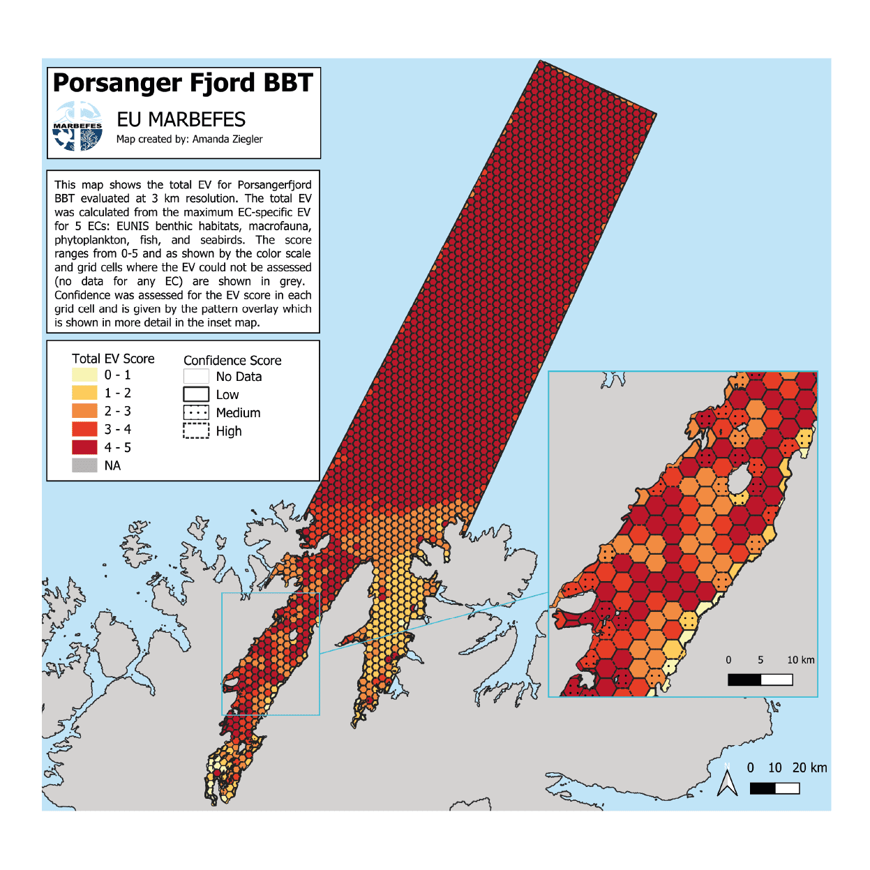
The Ecological Value Assessment (EVA) assesses the ecological value of the qualities of the marine ecosystem and their spatial distribution in an area. Starting from the original marine biological valuation approach (Derous et al., 2007), the EVA method has been further developed and tested in MARBEFES for wider applicability and flexibility. The method adopts an eco-centric perspective, whereby the ecological value (EV) is defined as the inherent (non-monetary) value of the qualities of an ecosystem, regardless of its anthropogenic use or social interests. EVA provides a harmonised, transparent, and flexible approach to combine multiple ecological metrics into a single, spatially explicit index of ecological value. Its purpose is to support decision-making in conservation, marine spatial planning, and ecosystem-based management by quantifying where biodiversity holds the highest ecological significance.
Aspects such as biodiversity, rarity and functions performed by multiple ecosystem components (EC) contribute to determine the ecological value of an area. EVA is essentially a multimetric index, where multiple metrics (AQs) are measured to account for these different values. The method is applied within a grid-based spatial framework, whereby each grid cell within an area is assigned scores resulting from the metric calculations. These are based on monitoring data or data-derived evidence of the distribution of the ecosystem components, but expert-based proxies may be used instead, where data are scarce or not available. The scores are aggregated into a composite index (EV), which can be visualised as ecological value maps, which can be used to identify hotspots of biodiversity importance and priority areas for management.
A key phase of the EVA method is the confidence assessment. This accounts for the multiple sources of uncertainty associated with the evidence used (e.g., whether data or expert judgement, whether quantitative or qualitative data, data consistency/coverage) and the assessment itself (e.g., number of AQ metrics measured). The output is a confidence map that is to be read alongside the EV map in order to inform on the confidence associated with the EVA results.
Limitations include dependency on available data and the challenge of weighting indicators across different ecological contexts. The EVA method is currently designed based on biodiversity at the community and ecosystem levels (e.g., ecosystem components defined as groups of species or habitat types) as this is the most common type of evidence available for the assessment (e.g., from ecological monitoring programmes). However, the method has the potential of being applied considering variable levels of biological organisation, e.g., accounting for the diversity of genes, biological traits (closely associated with functions) and habitat function metrics. This would require only minor adjustments (redefinition of the features of interest for the assessment) while the overall structure of the approach would remain the same.
EVA represents a robust, science-based tool to bring biodiversity value into policy and planning in line with the EU Biodiversity Strategy 2030.
The EVA tools
The implementation of EVA is divided into three phases (for details see guidance document):
Phase 1 – Preparatory work, where (a) the spatial system for the study area is defined (area boundaries and spatial grids), (b) the relevant data are identified and selected for the study area (ecosystem components, type of data, spatial and temporal consistency) and pre-processed for integration into the selected spatial system (this requires mapping, aggregation, possible modelling etc), (c) the key features of interest in the dataset (e.g., nationally rare species, biogenic habitats) are identified for the assessment.
Phase 2 – Ecological value calculation, where (a) the spatialised (gridded) data for the different ecosystem components are analysed to calculate key metrics (AQs) and aggregate them into ecological value scores (EV) for each individual ecosystem component and then across ecosystem components; (b) the results are mapped into the spatial system for the study area.
Phase 3 – information about the data used and the assessment undertaken is used (a) to calculate a confidence score associated with the EV results and (b) to map it in the spatial system for the study area.
Multiple tools are provided to help the user implementing EVA in full or in part:
The EVA-Excel tool implements the EV calculations as per Phase 2(a) above in an Excel environment. The preparatory work (Phase 1), final mapping of the results (Phase 2(b)) and confidence assessment (Phase 3) are not implemented by this tool.
Input required: • gridded dataset (table) on qualitative (presence /absence) or quantitative evidence (e.g., species abundance, habitat extent), separately for each of the ecosystem component s to be assessed; • user’s selection of the features of interest in the dataset.
Output: • gridded datasets (tables) of resulting AQs and EV for each ecosystem component assessed, and total EV (when results for multiple ecosystem components are combined).
Skills required for the tool implementation: • Ecological knowledge and understanding of the ecosystem components in the study area. • Knowledge and understanding of the ecological data available (for consideration, selection and pre-processing) • Basic knowledge of Excel. (Note that additional skills, e.g. GIS mapping, may be required to prepare the input data and map the outputs of the tool).
Tool instructions: Instructions for the use of the tool are given in the sheet ‘READ ME’ in the EVA-Excel tool.
The EVA-R tool implements the EV preparations, calculations and mapping as per Phases 1-3 above in an R environment.
Input required:
• georeferenced dataset (table including latitude and longitude) on qualitative (presence /absence) or quantitative evidence (e.g., species abundance, habitat extent), separately for each of the ecosystem components to be assessed;
• user’s selection of the features of interest in the dataset;
• the region of interest outline (geo-file) and optionally the geo-spatial grid (if no grid is provided, a grid will be created by the script).
Output:
• gridded datasets (tables) of resulting AQs and EV for each ecosystem component assessed, and total EV (across ecosystem components).
Skills required for the tool implementation:
• Ecological knowledge and understanding of the ecosystem components in the study area.
• Knowledge and understanding of the ecological data available (for consideration, selection and pre-processing)
• Knowledge of Rmarkdown.
Category:
Subcategory:
Tool Types:
Target User:
Level of uncertainty:
Version:
Rights:
Publication:
Difficulty:
Skill Required:
Authors:
Tool Contributors:
Project general coordinator:
Project Scientific manager:
Project Manager: